Optimal Control of a Double Cart-Pole System using CasADi

casadi
optimal-control
direct-collocation
Author

Edwin Reuvers

Published

23 August 2026

Introduction

I have previously used CasADi to optimise the length trajectory of a Hill-type muscle–tendon complex (MTC), maximising its average mechanical power output over a periodic cycle (see https://doi.org/10.1371/journal.pcbi.1014587). For this purpose I practiced with some examples to gain experience with optimal control and direct collocation in CasADi.

One of the examples I practice with is that of of a double cart-pole. This system consists of a cart and two pendulum links connected in series. The goal is to bring both pendulums from their hanging configuration to rest in the upright configuration, using only a horizontal force on the cart. Here, the manoeuvre must be completed in three seconds while minimising the integral of the squared cart force and keeping the cart within the track limits.

Although the setup is simple, the system is underactuated: the pendulum joints are passive, so their motion must be generated indirectly through the movement of the cart. The optimiser must find a force trajectory that exploits the coupled nonlinear dynamics to swing both pendulums upwards and bring the system to rest.

In this post, I formulate the optimal-control problem, explain how direct collocation turns it into a finite-dimensional optimisation problem, and implement it in CasADi using IPOPT. I then examine the resulting motion. For readers interested in the mechanics, the final section derives the equations of motion using both Lagrangian and Newton–Euler formulations.

System description

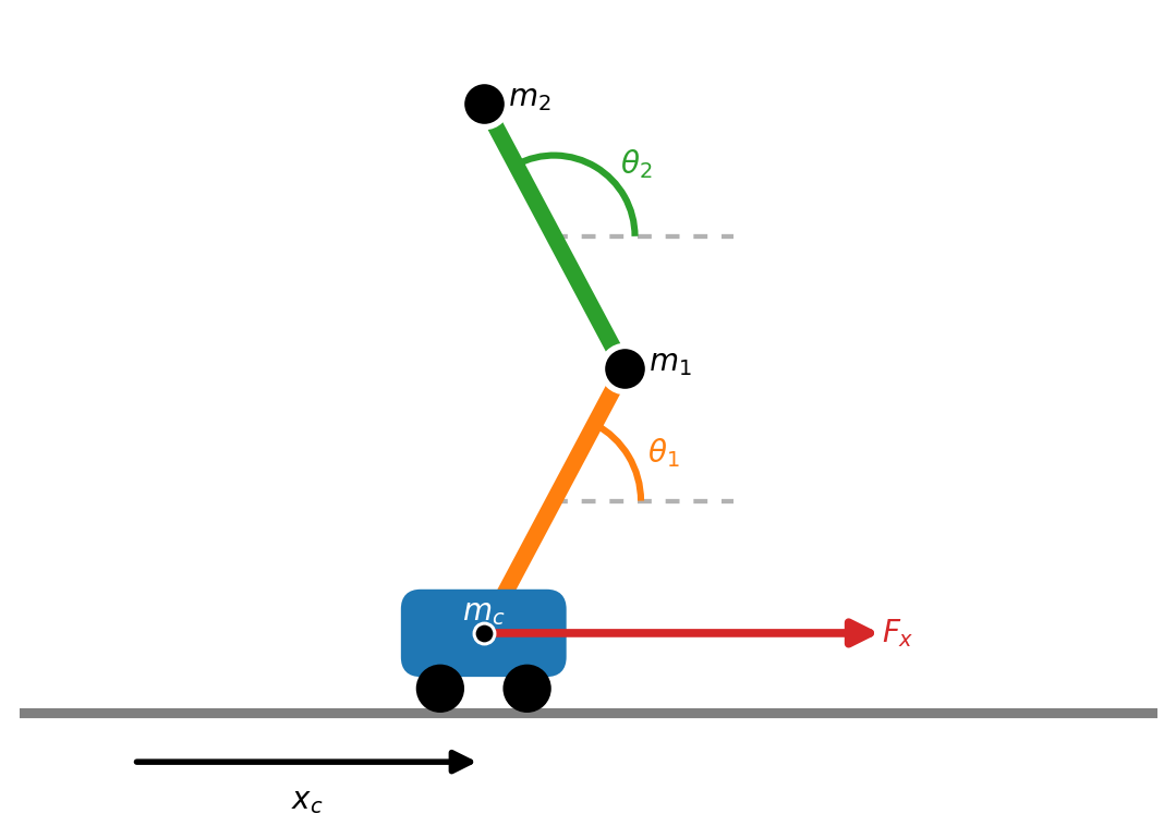
The system consists of a cart moving along a horizontal track with two pendulum links attached in series.

The cart has mass \(m_c\). The pendulum links are assumed massless and carry point masses \(m_1\) and \(m_2\) at their endpoints. The corresponding link lengths are \(l_1\) and \(l_2\).

The generalised coordinates are:

\[ q= \begin{bmatrix} x_c\\ \theta_1\\ \theta_2 \end{bmatrix} \]

where \(x_c\) is the cart position and \(\theta_1,\theta_2\) are the pendulum angles from the positive \(x\)-axis.

The state vector is:

\[ x= \begin{bmatrix} x_c\\ \theta_1\\ \theta_2\\ \dot{x}_c\\ \dot{\theta}_1\\ \dot{\theta}_2 \end{bmatrix} \]

The only control input is a horizontal force applied to the cart:

\[ u=F_x \]

The objective is to find an input trajectory that moves the system from the stable hanging configuration to the unstable upright configuration in a fixed time whilst minimising a certain control effort.

Double cart-pole coordinates, states, masses and control force.
Quantity Value Description
\(m_c\) \(0.5\ \mathrm{kg}\) Cart mass
\(m_1,m_2\) \(1.0\ \mathrm{kg}\) Pendulum point masses
\(l_1,l_2\) \(1.0\ \mathrm{m}\) Pendulum lengths
\(g\) \(9.81\ \mathrm{m\,s^{-2}}\) Gravitational acceleration
\(T\) \(3.0\ \mathrm{s}\) Fixed time horizon
\(x_{c,\max}\) \(2.0\ \mathrm{m}\) Absolute cart-position limit

Problem formulation

The goal is to find a state trajectory \(x(t)\) and control input \(u(t)\) that move the double cart-pole from the hanging configuration to the upright configuration over the fixed horizon \(T=3\ \mathrm{s}\). The objective is to minimise the integral of the squared cart force, subject to the system dynamics, prescribed initial and final states, and cart-position limits. The optimal-control problem is formulated as:

\[ \begin{aligned} \min_{x(\cdot),\,u(\cdot)}\quad &J=\int_0^T u(t)^2\,\mathrm{d}t &&\text{(objective function)} \\[4pt] \text{subject to}\quad &\dot{x}(t)=f(x(t),u(t)) &&\text{(dynamic constraints)} \\[4pt] &x(0)= \begin{bmatrix} 0\\-\pi/2\\-\pi/2\\0\\0\\0 \end{bmatrix}, \quad x(T)= \begin{bmatrix} 0\\\pi/2\\\pi/2\\0\\0\\0 \end{bmatrix} &&\text{(boundary constraints)} \\[4pt] &-x_{c,\max}\leq x_c(t)\leq x_{c,\max} &&\text{(path constraints)} \end{aligned} \]

Here, \(x_{c,\max}=2\ \mathrm{m}\), and the dynamic and path constraints apply throughout \(t\in[0,T]\). The dynamic constraints are described in the following subsection.

Dynamic constraints

The dynamic constraints require the state trajectory to satisfy the nonlinear equations of motion throughout the manoeuvre. With \(x=[q^T,\dot q^T]^T\), the first-order state dynamics are:

\[ \dot x=f(x,u)= \begin{bmatrix} \dot q\\ M(q)^{-1}\bigl(Q(u)-h(q,\dot q)\bigr) \end{bmatrix} \]

This follows from the standard mechanical form:

\[ M(q)\ddot q+h(q,\dot q)=Q(u) \]

where \(M(q)\) is the configuration-dependent inertia matrix, \(h(q,\dot q)\) contains gravity and velocity-dependent nonlinear terms, and \(Q(u)\) contains the generalised input forces. The horizontal cart force is the only control input; both pendulum joints are passive.

In the implementation, the accelerations are obtained by solving the linear system \(M(q)\ddot q=Q(u)-h(q,\dot q)\) directly, without explicitly forming \(M(q)^{-1}\).

The inertia matrix is:

\[ M(q)= \begin{bmatrix} m_c+m_1+m_2 & -l_1(m_1+m_2)\sin(\theta_1) & -l_2m_2\sin(\theta_2) \\ -l_1(m_1+m_2)\sin(\theta_1) & l_1^2(m_1+m_2) & l_1l_2m_2\cos(\theta_1-\theta_2) \\ -l_2m_2\sin(\theta_2) & l_1l_2m_2\cos(\theta_1-\theta_2) & l_2^2m_2 \end{bmatrix} \]

The nonlinear term is:

\[ h(q,\dot q)= \begin{bmatrix} -l_1(m_1+m_2)\dot{\theta}_1^2\cos(\theta_1) -l_2m_2\dot{\theta}_2^2\cos(\theta_2) \\ l_1 \left( g(m_1+m_2)\cos(\theta_1) +l_2m_2\dot{\theta}_2^2 \sin(\theta_1-\theta_2) \right) \\ l_2m_2 \left( g\cos(\theta_2) -l_1\dot{\theta}_1^2 \sin(\theta_1-\theta_2) \right) \end{bmatrix} \]

\(Q\) is:

\[ Q= \begin{bmatrix} u\\ 0\\ 0 \end{bmatrix} \]

The equations of motion are derived at the end of this post using both Lagrangian and Newton–Euler formulations.

CasADi implementation

The optimal-control problem is implemented in CasADi using direct collocation and solved with IPOPT. The system model is defined in dynamics.py, while visualize.py contains the animation utilities.

Dynamics
"""Dynamics models used by the optimal-control examples."""

import casadi as ca


def double_cartpole(state, force, parameters):
    """Return the first-order dynamics of the double cart-pole."""

    mc = parameters["mc"]
    g = parameters["g"]
    m1 = parameters["m1"]
    m2 = parameters["m2"]
    l1 = parameters["l1"]
    l2 = parameters["l2"]

    x_c, theta1, theta2, x_cdot, theta1dot, theta2dot = ca.vertsplit(state)

    sin = ca.sin
    cos = ca.cos

    M = ca.MX.zeros(3, 3)
    M[0, 0] = mc + m1 + m2
    M[0, 1] = -l1 * (m1 + m2) * sin(theta1)
    M[0, 2] = -l2 * m2 * sin(theta2)

    M[1, 0] = M[0, 1]
    M[1, 1] = l1**2 * (m1 + m2)
    M[1, 2] = l1 * l2 * m2 * cos(theta1 - theta2)

    M[2, 0] = M[0, 2]
    M[2, 1] = M[1, 2]
    M[2, 2] = l2**2 * m2

    h = ca.vertcat(
        -l1 * (m1 + m2) * theta1dot**2 * cos(theta1)
        - l2 * m2 * theta2dot**2 * cos(theta2),
        l1
        * (
            g * (m1 + m2) * cos(theta1)
            + l2 * m2 * theta2dot**2 * sin(theta1 - theta2)
        ),
        l2
        * m2
        * (g * cos(theta2) - l1 * theta1dot**2 * sin(theta1 - theta2)),
    )

    qdd = ca.solve(M, ca.vertcat(force, 0, 0) - h)
    return ca.vertcat(x_cdot, theta1dot, theta2dot, qdd)
Visualize
"""Visualisation utilities used by the optimal-control examples."""

from __future__ import annotations

import matplotlib.animation as animation
import matplotlib.pyplot as plt
from matplotlib.patches import Circle, FancyArrowPatch, FancyBboxPatch
import numpy as np


COLORS = {
    "background": "white",
    "ink": "black",
    "muted": "0.40",
    "rail": "0.50",
    "cart": "C0",
    "cart_edge": "C0",
    "force": "C3",
    "link_1": "C1",
    "link_2": "C2",
    "mass_1": "black",
    "mass_2": "black",
    "trace": "0.5",
}


def double_cartpole_trajectory(
    x,
    tend,
    dt,
    segparms,
    pause=0.0,
    *,
    control=None,
    colors=None,
    width=None,
    height=None,
    show=True,
    repeat=True,
    hud=True,
    static=False,
):
    """Visualize a double cart-pole trajectory.

    Parameters
    ----------
    x : array-like, shape (6, n_frames)
        Rows contain ``x_c, theta_1, theta_2`` and their velocities.
    tend : float
        Duration of the optimized trajectory in seconds.
    dt : float
        Sampling interval between the supplied states.
    segparms : mapping
        Must contain ``l1`` and ``l2``; masses are used to scale the markers.
    pause : float, optional
        Number of seconds for which the final pose remains visible.
    control : array-like, optional
        Horizontal cart force. Supply one value per state or per interval.
    colors : mapping, optional
        Colour palette. Missing entries are taken from ``COLORS``.
    width, height : float, optional
        Figure size in inches. Set either width or height; the other dimension
        is inferred from the trajectory bounds. If neither is set, width is
        10 inches. The supplied dimension is respected exactly.
    show : bool, optional
        Call ``plt.show()`` before returning.
    repeat : bool, optional
        Repeat the animation after the last frame. Enabled by default.
    hud : bool, optional
        Show the time and force badge.
    static : bool, optional
        Render the first frame as a normal Matplotlib figure without creating
        a ``FuncAnimation``. Returns ``(figure, axes)`` in this mode.

    Returns
    -------
    matplotlib.animation.FuncAnimation or tuple
        Animation by default; ``(figure, axes)`` when ``static=True``.
    """

    states = np.asarray(x, dtype=float)
    duration = float(tend)
    parameters = segparms
    palette = COLORS | ({} if colors is None else dict(colors))
    if states.ndim != 2 or states.shape[0] < 3:
        raise ValueError("states must have shape (at least 3, n_frames)")
    if states.shape[1] < 2:
        raise ValueError("at least two trajectory frames are required")
    if dt <= 0:
        raise ValueError("dt must be positive")

    l1 = float(parameters["l1"])
    l2 = float(parameters["l2"])
    m1 = float(parameters.get("m1", 1.0))
    m2 = float(parameters.get("m2", 1.0))

    original_frame_count = states.shape[1]

    if control is None:
        force = np.zeros(original_frame_count)
        show_force = False
    else:
        force = np.asarray(control, dtype=float).reshape(-1)
        if force.size == original_frame_count - 1:
            force = np.append(force, force[-1])
        elif force.size != original_frame_count:
            raise ValueError(
                "control must contain one value per state or per interval"
            )
        show_force = True

    # Repeat the final state and force to create a deliberate end pause.
    extra_frames = max(0, int(round(float(pause) / dt)))
    if extra_frames:
        final_state = np.repeat(states[:, -1:], extra_frames, axis=1)
        states = np.hstack((states, final_state))
        force = np.append(force, np.repeat(force[-1], extra_frames))

    x_c = states[0]
    theta1 = states[1]
    theta2 = states[2]

    x1 = x_c + l1 * np.cos(theta1)
    y1 = l1 * np.sin(theta1)
    x2 = x1 + l2 * np.cos(theta2)
    y2 = y1 + l2 * np.sin(theta2)

    cart_width = 0.48
    cart_height = 0.22
    wheel_radius = 0.075
    rail_y = -cart_height / 2 - 2.1 * wheel_radius

    # Leave room for the force arrow when the cart reaches a trajectory bound.
    horizontal_margin = 1.25
    x_min = min(np.min(x_c), np.min(x1), np.min(x2)) - horizontal_margin
    x_max = max(np.max(x_c), np.max(x1), np.max(x2)) + horizontal_margin
    y_min = min(rail_y - 0.35, np.min(y1), np.min(y2)) - 0.25
    y_max = max(cart_height, np.max(y1), np.max(y2)) + 0.35

    data_width = max(x_max - x_min, 1e-9)
    data_height = max(y_max - y_min, 1e-9)
    data_aspect = data_width / data_height
    # Preserve enough canvas for the badges and axis labels even when
    # the physical trajectory itself is extremely narrow or wide.
    figure_aspect = float(np.clip(data_aspect, 1.35, 2.0))

    # Match the data limits to the canvas aspect ratio. Without this padding,
    # ``aspect="equal"`` shrinks the axes box when the horizontal trajectory
    # range is small, leaving unused space at either side of the figure.
    if data_aspect < figure_aspect:
        extra_width = data_height * figure_aspect - data_width
        x_min -= extra_width / 2
        x_max += extra_width / 2
    elif data_aspect > figure_aspect:
        extra_height = data_width / figure_aspect - data_height
        y_min -= extra_height / 2
        y_max += extra_height / 2

    if width is None and height is None:
        width = 10.0
    if width is not None and width <= 0:
        raise ValueError("width must be positive")
    if height is not None and height <= 0:
        raise ValueError("height must be positive")
    if width is None:
        width = float(height) * figure_aspect
    elif height is None:
        height = float(width) / figure_aspect

    fig, ax = plt.subplots(
        figsize=(float(width), float(height)),
        constrained_layout=True,
    )
    # Transparent canvas: it appears white in a normal window and blends into
    # the background when embedded in a webpage or exported with transparency.
    fig.patch.set_facecolor(palette["background"])
    fig.patch.set_alpha(0)
    ax.set_facecolor("none")
    ax.set_xlim(x_min, x_max)
    ax.set_ylim(y_min, y_max)
    ax.set_aspect("equal", adjustable="box")
    ax.set_xlabel(r"cart position $x_c$ [m]")
    ax.set_ylabel("height [m]")
    ax.tick_params(colors=palette["muted"], length=0)
    ax.grid(axis="y", color=palette["ink"], alpha=0.07, linewidth=0.8)
    for spine in ax.spines.values():
        spine.set_visible(False)

    # A single neutral rail provides a clean reference for cart motion.
    ax.axhline(rail_y, color=palette["rail"], linewidth=3.0, zorder=1)

    trace, = ax.plot(
        [], [],
        color=palette["trace"],
        linewidth=1.8,
        alpha=0.6,
        linestyle=(0, (2, 3)),
        zorder=2,
    )
    link1, = ax.plot(
        [], [],
        color=palette["link_1"],
        linewidth=5,
        solid_capstyle="round",
        zorder=5,
    )
    link2, = ax.plot(
        [], [],
        color=palette["link_2"],
        linewidth=5,
        solid_capstyle="round",
        zorder=5,
    )

    mass_scale = 190
    mass1 = ax.scatter(
        [], [], s=mass_scale * np.sqrt(max(m1, 0.05)),
        color=palette["mass_1"], edgecolor="white", linewidth=1.8, zorder=7,
    )
    mass2 = ax.scatter(
        [], [], s=mass_scale * np.sqrt(max(m2, 0.05)),
        color=palette["mass_2"], edgecolor="white", linewidth=1.8, zorder=7,
    )
    pivot = ax.scatter(
        [], [], s=38, color=palette["ink"], edgecolor="white",
        linewidth=1.0, zorder=8,
    )

    cart = FancyBboxPatch(
        (0, 0),
        cart_width,
        cart_height,
        boxstyle="round,pad=0.025,rounding_size=0.055",
        linewidth=2,
        edgecolor=palette["cart_edge"],
        facecolor=palette["cart"],
        zorder=6,
    )
    ax.add_patch(cart)

    wheel_left = Circle((0, 0), wheel_radius, color=palette["ink"], zorder=7)
    wheel_right = Circle((0, 0), wheel_radius, color=palette["ink"], zorder=7)
    ax.add_patch(wheel_left)
    ax.add_patch(wheel_right)

    force_arrow = FancyArrowPatch(
        (0, 0),
        (0, 0),
        arrowstyle="-|>",
        mutation_scale=16,
        linewidth=2.5,
        color=palette["force"],
        # Above the cart body, but below the black center-of-mass marker.
        zorder=7.5,
    )
    force_arrow.set_visible(show_force)
    ax.add_patch(force_arrow)

    time_text = ax.text(
        0.98, 0.90, "",
        transform=ax.transAxes,
        ha="right",
        va="top",
        fontsize=11,
        color=palette["ink"],
        bbox={
            "boxstyle": "round,pad=0.3",
            "facecolor": "white",
            "edgecolor": "none",
            "alpha": 0.72,
        },
    )
    force_text = ax.text(
        0.98, 0.82, "",
        transform=ax.transAxes,
        ha="right",
        va="top",
        fontsize=11,
        fontweight="bold",
        color=palette["force"],
    )
    force_text.set_visible(show_force)

    if not hud:
        for artist in (
            time_text,
            force_text,
            trace,
        ):
            artist.set_visible(False)

    max_force = max(float(np.max(np.abs(force))), np.finfo(float).eps)
    max_arrow_length = (x_max - x_min) / 3

    def update(frame):
        cart_x = x_c[frame]
        cart.set_bounds(
            cart_x - cart_width / 2,
            -cart_height / 2,
            cart_width,
            cart_height,
        )
        wheel_y = -cart_height / 2 - wheel_radius
        wheel_left.center = (cart_x - 0.145, wheel_y)
        wheel_right.center = (cart_x + 0.145, wheel_y)

        link1.set_data([cart_x, x1[frame]], [0, y1[frame]])
        link2.set_data([x1[frame], x2[frame]], [y1[frame], y2[frame]])
        mass1.set_offsets([[x1[frame], y1[frame]]])
        mass2.set_offsets([[x2[frame], y2[frame]]])
        pivot.set_offsets([[cart_x, 0]])
        trace.set_data(x2[: frame + 1], y2[: frame + 1])

        current_force = force[frame]
        arrow_length = max_arrow_length * current_force / max_force
        if arrow_length > 0:
            arrow_length = min(arrow_length, x_max - cart_x - 0.05)
        elif arrow_length < 0:
            arrow_length = -min(-arrow_length, cart_x - x_min - 0.05)
        # Apply the force at the marked cart center of mass (x_c, 0).
        arrow_y = 0.0
        force_arrow.set_visible(show_force and abs(current_force) > 1e-8)
        force_arrow.set_positions(
            (cart_x, arrow_y),
            (cart_x + arrow_length, arrow_y),
        )
        force_text.set_text(rf"$F_x = {current_force:+5.1f}\,\mathrm{{N}}$")

        elapsed = min(frame * dt, float(duration))
        time_text.set_text(f"t = {elapsed:4.2f} s")

        return (
            cart,
            wheel_left,
            wheel_right,
            link1,
            link2,
            mass1,
            mass2,
            pivot,
            trace,
            time_text,
            force_arrow,
            force_text,
        )

    if static:
        update(0)
        if show:
            plt.show()
        return fig, ax

    ani = animation.FuncAnimation(
        fig,
        update,
        frames=states.shape[1],
        interval=1000 * dt,
        blit=True,
        repeat=repeat,
        repeat_delay=700,
    )

    # Draw the first pose immediately, which also makes static notebook output
    # and screenshots useful before the animation starts.
    update(0)
    if show:
        plt.show()

    return ani


def save_animation_gif(ani, filename, *, fps, dpi=300):
    """Save a Matplotlib animation as a looping GIF on a white canvas."""

    if fps <= 0:
        raise ValueError("fps must be positive")
    fig = ani._fig
    
    fig.patch.set_alpha(1)
    fig.patch.set_facecolor("white")
    writer = animation.PillowWriter(
        fps=fps,
        metadata={"title": "Double cart-pole swing-up"},
    )
    ani.save(filename, writer=writer, dpi=dpi)
import casadi as ca
import matplotlib.pyplot as plt
import numpy as np

import dynamics, visualize

do_ani = False # Do animation

# %% Parameters
segparms = {
    "mc": 0.5,  # [kg] cart mass
    "g": 9.81,  # [m/s^2] gravitational acceleration
    "m1": 1.0,  # [kg] first pendulum point mass
    "m2": 1.0,  # [kg] second pendulum point mass
    "l1": 1.0,  # [m] first link length
    "l2": 1.0,  # [m] second link length
}

tf = 3
xc_max = 2  # [m] bounds on absolute xc (i.e. -xc_max < xc < xc_max)

# %% Define symbolic state and control
x = ca.MX.sym("x", 6)
u = ca.MX.sym("u")

# %% Model dynamics
xdot = dynamics.double_cartpole(x, u, segparms)
f_dyn = ca.Function("f_dyn", [x, u], [xdot, u**2])

# %% Initialize
N = 100  # number of mesh intervals
opti = ca.Opti()

# Get collocation points
d = 3  # collocation polynomial degree
tau = ca.collocation_points(d, "radau")

# Collocation linear maps for inter- and extrapolation
C, D, B = ca.collocation_coeff(tau)

# Decision variables
x_k = opti.variable(6, N + 1)
u_k = opti.variable(1, N)

# %% Boundary constraints
# Initial constraints
x0 = np.array([0, -np.pi/2, -np.pi/2, 0, 0, 0])
opti.subject_to(x_k[:, 0] == x0)

# Final constraints
xend = np.array([0, np.pi/2, np.pi/2, 0, 0, 0])
opti.subject_to(x_k[:, -1] == xend)

# %% Path constraints
opti.subject_to(opti.bounded(-xc_max, x_k[0, :], xc_max))

# %% Initial guesses
theta1_init = np.linspace(x0[1], xend[1], N + 1)
theta2_init = np.linspace(x0[2], xend[2], N + 1)
opti.set_initial(x_k[0, :], 0)
opti.set_initial(x_k[1, :], theta1_init)
opti.set_initial(x_k[2, :], theta2_init)
opti.set_initial(x_k[3:6, :], 0)
opti.set_initial(u_k, 0)

# %% Formulate the NLP
J = 0
dt = tf / N
for i in range(N):
    # Collect and store states and controls
    Xk = x_k[:, i]
    Xk_next = x_k[:, i + 1]
    Uk = u_k[:, i]

    # States at midpoints
    Xc = opti.variable(6, d)
    opti.subject_to(opti.bounded(-xc_max, Xc[0, :], xc_max))
    # It helps to give a proper initial guess for these as well
    Xc_init = np.array([0, theta1_init[i], theta2_init[i], 0, 0, 0])
    opti.set_initial(Xc, np.tile(Xc_init, (d, 1)).T)

    # Dynamics
    ode, Jp = f_dyn(Xc, Uk)
    Z = ca.horzcat(Xk, Xc)  # Interpolation points of collocation polynomial
    Pidot = ca.mtimes(Z, C) / dt  # Slope of interpolating polynomial
    opti.subject_to(Pidot == ode)  # Match the ODE right-hand side
    X_end = ca.mtimes(Z, D)  # State at the end of the interval
    opti.subject_to(X_end == Xk_next)  # Continuity constraint

    # Compute cost
    J = J + ca.mtimes(Jp, B) * dt

# %% Solve
opti.minimize(J)
opti.solver("ipopt")
sol = opti.solve()

# %% Extract solution
t_sol = np.linspace(0, tf, N + 1)
x_sol = sol.value(x_k)
u_sol = sol.value(u_k)

# %% Animation
if do_ani:
    ani = visualize.double_cartpole_trajectory(
        x_sol,
        tf,
        dt,
        segparms,
        pause=1,
        width=6,
        control=u_sol,
        show=False,
    )
    
    visualize.save_animation_gif(ani, "double_cartpole_swingup.gif", fps=max(1, round(1 / dt)))

# %% Save blog assets
fig, axs = plt.subplots(2, 2, figsize=(6, 4), sharex=True, constrained_layout=True)
axs[0,0].plot(t_sol, x_sol[0], c='C0')
axs[0,0].set_ylabel(r"$x_c$ [m]")
axs[0,1].plot(t_sol, x_sol[1], c='C1')
axs[0,1].set_ylabel(r"$\theta_1$ [rad]")
axs[1,0].plot(t_sol, x_sol[2], c='C2')
axs[1,0].set_ylabel(r"$\theta_2$ [rad]")
axs[1,1].step(t_sol[:-1], u_sol, where="post", color="C3")
axs[1,1].set_ylabel(r"$F_x$ [N]")
for ax in axs.flat:
    ax.grid(alpha=0.2)
    ax.set_xlabel("Time [s]")
fig.savefig("double_cartpole_swingup_trajectories.png", dpi=600, transparent=True, bbox_inches="tight")
plt.show()

Results

For the fixed horizon \(T=3\ \mathrm{s}\), IPOPT converges to a control-effort objective of:

\[ J^\star=292.57\ \mathrm{N^2\,s} \]

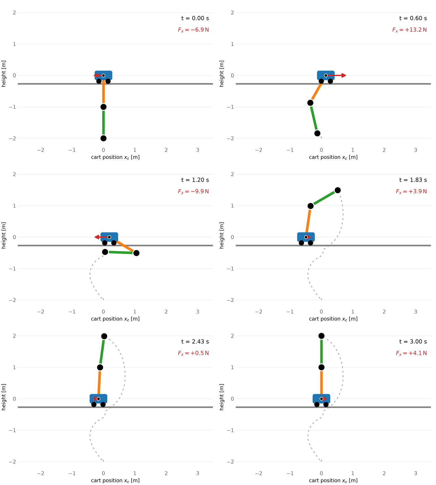
The resulting swing-up trajectory is shown below. The optimiser distributes the cart force over the available time whilst using the nonlinear coupling to raise both pendulums to the upright equilibrium.

Control-effort-optimal swing-up obtained with direct collocation and IPOPT.

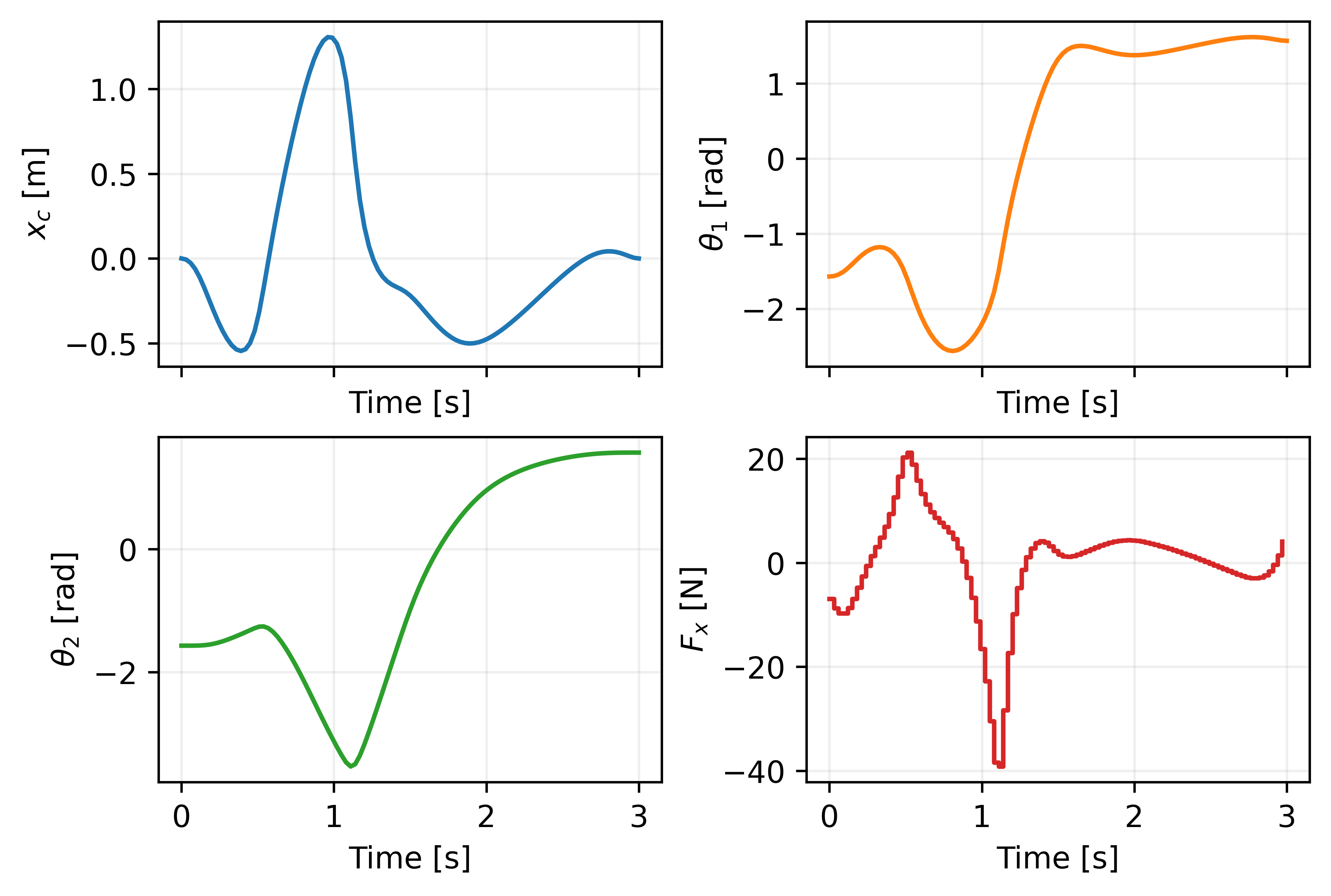
The state and input trajectories show how the cart motion generates the required pendulum motion. Both angles reach \(\pi/2\), whilst the cart position and all velocities return to zero at the final time.

Optimised states and cart force over the fixed time horizon.

Derivation of the equations of motion

The geometry and angle convention are shared by both derivations below. The first uses energy, while the second uses Cartesian force balances and virtual work. Both lead to the same \(M(q)\) and \(h(q,\dot q)\) used above.

Shared coordinates and kinematics

Collect the generalised coordinates and their derivatives as

\[ q=\begin{bmatrix}x_c\\\theta_1\\\theta_2\end{bmatrix},\qquad \dot q=\begin{bmatrix}\dot x_c\\\dot\theta_1\\\dot\theta_2\end{bmatrix},\qquad \ddot q=\begin{bmatrix}\ddot x_c\\\ddot\theta_1\\\ddot\theta_2\end{bmatrix}. \]

The masses are \(m_c,m_1,m_2\), the link lengths are \(l_1,l_2\), and \(g>0\). Both angles are absolute angles measured from the positive world \(x\)-axis.

Positions and velocities

The mass positions in the fixed world frame are

\[ p_c=\begin{bmatrix}x_c\\0\end{bmatrix},\qquad p_1=\begin{bmatrix}x_c+l_1\cos\theta_1\\l_1\sin\theta_1\end{bmatrix}, \]

\[ p_2=\begin{bmatrix} x_c+l_1\cos\theta_1+l_2\cos\theta_2\\ l_1\sin\theta_1+l_2\sin\theta_2 \end{bmatrix}. \]

For each mass, define the position Jacobian

\[ J_i(q)=\frac{\partial p_i}{\partial q}. \]

The Cartesian velocities then follow from the chain rule:

\[ v_i=J_i(q)\dot q. \]

Lagrange formulation

Lagrangian mechanics derives the model from kinetic and potential energy.

Kinetic and potential energy

Because the links are massless, the total kinetic energy is the sum of the translational kinetic energies:

\[ T=\frac12m_c\,v_c^Tv_c +\frac12m_1v_1^Tv_1 +\frac12m_2v_2^Tv_2. \]

With the world \(y\)-axis pointing upwards, the gravitational potential energy is

\[ V=m_1g\,p_{1,y}+m_2g\,p_{2,y}. \]

Using the positions above,

\[ V=g\left[l_1(m_1+m_2)\sin\theta_1 +l_2m_2\sin\theta_2\right]. \]

Lagrangian and Euler–Lagrange equation

The Lagrangian is

\[ L(q,\dot q)=T(q,\dot q)-V(q). \]

The equations of motion follow from

\[ \frac{d}{dt}\left(\frac{\partial L}{\partial\dot q}\right) -\frac{\partial L}{\partial q} =Q_\mathrm{external}. \]

The time derivative of the generalised momentum is expanded with the chain rule:

\[ \frac{d}{dt}\left(\frac{\partial L}{\partial\dot q}\right) = \frac{\partial}{\partial q} \left(\frac{\partial L}{\partial\dot q}\right)\dot q + \frac{\partial}{\partial\dot q} \left(\frac{\partial L}{\partial\dot q}\right)\ddot q. \]

This separates the acceleration-dependent part from all remaining terms.

Extracting \(M(q)\) and \(h(q,\dot q)\)

The coefficient of \(\ddot q\) is the mass matrix:

\[ \boxed{ M(q)= \frac{\partial}{\partial\dot q} \left(\frac{\partial L}{\partial\dot q}\right) =\frac{\partial^2L}{\partial\dot q^2} }. \]

Since the potential energy does not depend on \(\dot q\), this is equivalently the velocity Hessian of the kinetic energy:

\[ M(q)=\frac{\partial^2T}{\partial\dot q^2}. \]

Everything remaining on the left-hand side forms \(h\):

\[ \boxed{ h(q,\dot q)= \frac{\partial}{\partial q} \left(\frac{\partial L}{\partial\dot q}\right)\dot q -\frac{\partial L}{\partial q} }. \]

Thus \(M\) contains the inertial coefficients, while \(h\) contains the gravity, Coriolis, and centrifugal terms.

Complete equation of motion

The horizontal input force acts only on the cart:

\[ Q_\mathrm{external}=\begin{bmatrix}u\\0\\0\end{bmatrix}. \]

Substitution into the Euler–Lagrange equation gives the required standard mechanical form:

\[ M(q)\ddot q+h(q,\dot q) =\begin{bmatrix}u\\0\\0\end{bmatrix}. \]

Newton–Euler formulation

The same model can be obtained directly from Cartesian accelerations and forces.

Using the same positions and Jacobians as above, the Cartesian accelerations follow from the product rule:

\[ a_i=J_i\ddot q+\dot J_i\dot q,\qquad \dot J_i=\sum_{k=1}^{3}\frac{\partial J_i}{\partial q_k}\dot q_k. \]

This split is useful because \(J_i\ddot q\) contains the acceleration-dependent terms, while \(\dot J_i\dot q\) contains the nonlinear velocity terms.

Newton residuals and gravity

Gravity acts on the two point masses as

\[ F_{g,1}=\begin{bmatrix}0\\-m_1g\end{bmatrix},\qquad F_{g,2}=\begin{bmatrix}0\\-m_2g\end{bmatrix}. \]

Writing Newton’s law as a residual gives

\[ R_c=m_c a_c,\qquad R_1=m_1a_1-F_{g,1},\qquad R_2=m_2a_2-F_{g,2}. \]

The vertical weight of the cart is balanced by its normal force and does not contribute to the permitted horizontal motion.

Projection using the transposed Jacobian

The residuals above are Cartesian vectors. To obtain equations in \(q\), project them onto the generalised coordinates. From virtual work,

\[ \delta p_i=J_i\delta q, \qquad F_i^T\delta p_i=(J_i^TF_i)^T\delta q, \]

so a Cartesian force contributes the generalised force \(J_i^TF_i\). Applying this projection to the Newton residuals gives

\[ Q_\mathrm{internal} =J_c^TR_c+J_1^TR_1+J_2^TR_2. \]

This projection also eliminates the internal joint reaction forces: their virtual-work contributions cancel.

Complete equation of motion

The horizontal input force acts only on the cart:

\[ Q_\mathrm{external}=\begin{bmatrix}u\\0\\0\end{bmatrix}. \]

The equations of motion can therefore be written as the residual

\[ R(q,\dot q,\ddot q,u) =Q_\mathrm{internal}-Q_\mathrm{external}=0. \]

Extracting \(M(q)\) and \(h(q,\dot q)\)

After substituting \(a_i=J_i\ddot q+\dot J_i\dot q\), the projected internal term is affine in \(\ddot q\):

\[ Q_\mathrm{internal}=M(q)\ddot q+h(q,\dot q). \]

The mass matrix is therefore the coefficient matrix of \(\ddot q\):

\[ \boxed{ M(q)=\frac{\partial Q_\mathrm{internal}}{\partial\ddot q} }. \]

To obtain \(h\), set all generalised accelerations to zero in \(Q_\mathrm{internal}\):

\[ \boxed{ h(q,\dot q) =Q_\mathrm{internal}(q,\dot q,0) }. \]

Extracting both terms before subtracting \(Q_\mathrm{external}\) keeps the control input separate from the mechanical terms by construction. The full residual is then

\[ R=M(q)\ddot q+h(q,\dot q)-Q_\mathrm{external}. \]

Setting \(R=0\) gives the required standard mechanical form:

\[ M(q)\ddot q+h(q,\dot q) =\begin{bmatrix}u\\0\\0\end{bmatrix}. \]

Lagrange script

"""Lagrange derivation for a double cart-pole.

The derivation follows the Lagrange formulation in the "Mathematical
derivation" callout of ``index.qmd``. The numbered code cells follow the same
order as the relevant sections and subsections in that callout.

The result has the standard mechanical form

    M(q) qdd + h(q, qd) = Q_external.
"""

import sympy as sp


# %% 1. Coordinates, parameters, and conventions
# See "Shared coordinates and kinematics".
x_c, theta1, theta2 = sp.symbols("x_c theta_1 theta_2", real=True)
x_cd, theta1d, theta2d = sp.symbols("x_cdot theta_1dot theta_2dot", real=True)
x_cdd, theta1dd, theta2dd = sp.symbols(
    "x_cddot theta_1ddot theta_2ddot", real=True
)

q = sp.Matrix([x_c, theta1, theta2])
qd = sp.Matrix([x_cd, theta1d, theta2d])
qdd = sp.Matrix([x_cdd, theta1dd, theta2dd])

u = sp.symbols("u", real=True)
mc, m1, m2 = sp.symbols("m_c m_1 m_2", positive=True)
l1, l2 = sp.symbols("l_1 l_2", positive=True)
g = sp.symbols("g", positive=True)


# %% 2. Kinematics
# See "Shared coordinates and kinematics".
# Both pendulum angles are absolute angles measured from the positive x-axis.
p_cart = sp.Matrix([x_c, 0])
p1 = sp.Matrix([
    x_c + l1 * sp.cos(theta1),
    l1 * sp.sin(theta1),
])
p2 = sp.Matrix([
    x_c + l1 * sp.cos(theta1) + l2 * sp.cos(theta2),
    l1 * sp.sin(theta1) + l2 * sp.sin(theta2),
])

# For p_i(q), the chain rule gives v_i = J_i(q) qd.
J_cart = p_cart.jacobian(q)
J1 = p1.jacobian(q)
J2 = p2.jacobian(q)

v_cart = sp.simplify(J_cart * qd)
v1 = sp.simplify(J1 * qd)
v2 = sp.simplify(J2 * qd)


# %% 3. Kinetic and potential energy
# See "Lagrange formulation > Kinetic and potential energy".
# The links are massless, so the kinetic energy is purely translational.
T = sp.simplify(
    sp.Rational(1, 2) * mc * v_cart.dot(v_cart)
    + sp.Rational(1, 2) * m1 * v1.dot(v1)
    + sp.Rational(1, 2) * m2 * v2.dot(v2)
)

# With y pointing upward, gravitational potential energy is m_i*g*y_i.
V = sp.simplify(m1 * g * p1[1] + m2 * g * p2[1])


# %% 4. Lagrangian and Euler--Lagrange equation
# See "Lagrange formulation > Lagrangian and Euler--Lagrange equation".
L = sp.simplify(T - V)

# Generalized momentum and the configuration derivative of the Lagrangian.
dLdqd = L.diff(qd)
dLdq = L.diff(q)


# %% 5. Extracting M(q) and h(q, qd)
# See "Lagrange formulation > Extracting M(q) and h(q, qdot)".
#
# Expanding d/dt(dL/dqd) with the chain rule gives
#
#   d/dt(dL/dqd)
#       = jacobian(dLdqd, q) * qd + jacobian(dLdqd, qd) * qdd.
#
# The coefficient of qdd is M. Everything that remains on the left-hand side
# of the Euler--Lagrange equation is h.
M = sp.simplify(dLdqd.jacobian(qd))
h = sp.simplify(dLdqd.jacobian(q) * qd - dLdq)


# %% 6. Complete equation of motion
# See "Lagrange formulation > Complete equation of motion".
Q_external = sp.Matrix([u, 0, 0])
equations = sp.simplify(M * qdd + h - Q_external)

# Reconstruct the Euler--Lagrange left-hand side independently and verify that
# it equals M*qdd + h.
euler_lagrange = sp.simplify(
    dLdqd.jacobian(q) * qd
    + dLdqd.jacobian(qd) * qdd
    - dLdq
)
assert sp.simplify(euler_lagrange - (M * qdd + h)) == sp.zeros(3, 1)

M_lagrange = M
h_lagrange = h

if __name__ == "__main__":
    print("\n=== M(q) ===")
    sp.pprint(M_lagrange)
    print("\nLaTeX: ", sp.latex(M_lagrange))

    print("\n=== h(q, qdot) ===")
    sp.pprint(h_lagrange)
    print("\nLaTeX: ", sp.latex(h_lagrange))

    print("\n=== Q_external ===")
    sp.pprint(Q_external)
    print("\nSymbolic Euler--Lagrange reconstruction: OK")

Download double_cartpole_dynamics_lagrange.py.

Newton–Euler script

"""Newton--Euler derivation for a double cart-pole.

The derivation follows the Newton--Euler formulation in the "Mathematical
derivation" callout of ``index.qmd``. The numbered code cells follow the same
order as the relevant sections and subsections in that callout.

Model assumptions
-----------------
* The cart has mass m_c; the links are massless.
* m_1 and m_2 are point masses at the ends of the links.
* theta_1 and theta_2 are absolute angles measured from the positive x-axis.
* The only input is the horizontal force u acting on the cart.

The result has the standard mechanical form

    M(q) qdd + h(q, qd) = Q_external.
"""

import sympy as sp


# %% 1. Coordinates, parameters, and conventions
# See "Shared coordinates and kinematics".
#
# q, qd, and qdd are treated as independent symbolic vectors. This makes it
# straightforward to collect all coefficients multiplying qdd.
x_c, theta1, theta2 = sp.symbols("x_c theta_1 theta_2", real=True)
x_cd, theta1d, theta2d = sp.symbols("x_cdot theta_1dot theta_2dot", real=True)
x_cdd, theta1dd, theta2dd = sp.symbols("x_cddot theta_1ddot theta_2ddot", real=True)

q = sp.Matrix([x_c, theta1, theta2])
qd = sp.Matrix([x_cd, theta1d, theta2d])
qdd = sp.Matrix([x_cdd, theta1dd, theta2dd])

u = sp.symbols("u", real=True)
mc, m1, m2 = sp.symbols("m_c m_1 m_2", positive=True)
l1, l2 = sp.symbols("l_1 l_2", positive=True)
g = sp.symbols("g", positive=True)


# %% 2. Kinematics
# See "Shared coordinates and kinematics".
#
# Position kinematics
#
# All positions are expressed in the fixed world frame. Because the angles
# are absolute, the position of m_2 contains cos(theta2), not
# cos(theta1 + theta2).
p_cart = sp.Matrix([x_c, 0])
p1 = sp.Matrix([
    x_c + l1 * sp.cos(theta1),
    l1 * sp.sin(theta1),
])
p2 = sp.Matrix([
    x_c + l1 * sp.cos(theta1) + l2 * sp.cos(theta2),
    l1 * sp.sin(theta1) + l2 * sp.sin(theta2),
])


# Jacobians and velocities
#
# For every position p_i(q), v_i = J_i(q) qd, where J_i = d p_i / d q.
# The velocities are not used later in the derivation, but are included
# explicitly to make the chain rule visible.
J_cart = p_cart.jacobian(q)
J1 = p1.jacobian(q)
J2 = p2.jacobian(q)

v_cart = sp.simplify(J_cart * qd)
v1 = sp.simplify(J1 * qd)
v2 = sp.simplify(J2 * qd)


# Time derivative of a Jacobian
def time_derivative_of_jacobian(J):
    """Compute Jdot(q, qd) using the multivariable chain rule.

    Since J depends only on q, elementwise
        Jdot = sum_k (dJ/dq_k) * qd_k.
    """

    Jdot = sp.zeros(J.rows, J.cols)
    for row in range(J.rows):
        for col in range(J.cols):
            Jdot[row, col] = sum(
                sp.diff(J[row, col], q[k]) * qd[k]
                for k in range(len(q))
            )
    return sp.simplify(Jdot)


# Cartesian accelerations
#
# Applying the product rule to v_i = J_i qd:
#     a_i = J_i qdd + Jdot_i qd.
# The first part is linear in qdd; the second contains the nonlinear velocity
# contributions (centrifugal/Coriolis).
Jdot_cart = time_derivative_of_jacobian(J_cart)
Jdot1 = time_derivative_of_jacobian(J1)
Jdot2 = time_derivative_of_jacobian(J2)

a_cart = sp.simplify(J_cart * qdd + Jdot_cart * qd)
a1 = sp.simplify(J1 * qdd + Jdot1 * qd)
a2 = sp.simplify(J2 * qdd + Jdot2 * qd)


# %% 3. Newton residuals and gravity
# See "Newton--Euler formulation > Newton residuals and gravity".
#
# Write Newton's law as m_i*a_i - F_g,i = 0 (without external force).
# Gravity on the cart is omitted: its vertical motion is constrained and the
# vertical normal force balances its weight. These forces perform no virtual
# work in the permitted horizontal direction.
F_gravity1 = sp.Matrix([0, -m1 * g])
F_gravity2 = sp.Matrix([0, -m2 * g])

R_cart = mc * a_cart
R1 = m1 * a1 - F_gravity1
R2 = m2 * a2 - F_gravity2


# %% 4. Projection using the transposed Jacobian
# See "Newton--Euler formulation > Projection using the transposed Jacobian".
#
# Virtual work gives Q_i = J_i.T * F_i. The same projection converts the
# Cartesian Newton residuals into three generalized equations.
Q_internal = sp.simplify(
    J_cart.T * R_cart
    + J1.T * R1
    + J2.T * R2
)


# %% 5. Complete equation of motion
# See "Newton--Euler formulation > Complete equation of motion".
#
# Only x is actuated. Therefore equations = 0 is equivalent to
#     Q_internal = Q_external.
Q_external = sp.Matrix([u, 0, 0])
equations = sp.simplify(Q_internal - Q_external)


# %% 6. Extracting M(q) and h(q, qd)
# See "Newton--Euler formulation > Extracting M(q) and h(q, qdot)".
#
# Q_internal = M*qdd + h. Obtain M by differentiating with respect to qdd.
# Setting qdd = 0 in Q_internal then leaves h directly. Keeping the external
# force out of this extraction makes it explicit that h cannot depend on u.
M = sp.simplify(Q_internal.jacobian(qdd))
h = sp.simplify(Q_internal.subs(dict.fromkeys(qdd, 0)))

# Symbolically verify the exact reconstruction of the residual.
reconstruction_error = sp.simplify(equations - (M * qdd + h - Q_external))
assert reconstruction_error == sp.zeros(3, 1)


# Result and output
# Keep M_newton and h_newton as descriptive aliases for use from another
# script or notebook.
M_newton = M
h_newton = h

if __name__ == "__main__":
    print("\n=== M(q) ===")
    sp.pprint(M_newton)
    print("\nLaTeX: ", sp.latex(M_newton))

    print("\n=== h(q, qdot) ===")
    sp.pprint(h_newton)
    print("\nLaTeX: ", sp.latex(h_newton))

    print("\n=== Q_external ===")
    sp.pprint(Q_external)
    print("\nSymbolic reconstruction M*qdd + h - Q_external: OK")

Download double_cartpole_dynamics_newton_euler.py.